

When we first analyze any sample, we normally collect a Survey Spectrum as the first analysis. Survey Spectra reveal what elements are present within the detection limits of XPS. We need to know what elements are present and also how clean or dirty the sample is. For these reasons we normally collect a Survey Spectrum as the first analysis.
We likewise need to know if we are looking at the correct area or feature. We collect a survey spectrum to know if the customer gave us the correct sample or not. All of these “needs” are satisfied by collecting a Survey Spectrum. To achieve this goal we must fully identify and label each of the major peaks that we can see with our human eyes.
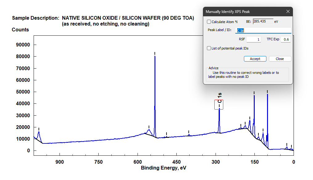
After we have processed a few Survey Spectra, we notice that the “as-received” surface of every sample has 2 photoelectron peaks at approximately the same BEs. These 2 peaks appear at ~285 eV and ~530 eV, which belong to Carbon and Oxygen, respectively. These 2 peaks are usually due to Adventitious Carbon Compounds, also known as Air-borne Molecular Contamination. If by chance your sample is an organic polymer, then the carbon and oxygen are very likely due to the bulk chemistry of the organic polymer.
Adventitious Carbon is never “pure carbon”, but rather a mixture of various types of Carbon, Hydrogen, and Oxygen based organic compounds that appear on the surface of every sample. Every sample has been exposed to the atmosphere of not only your laboratory, but also the container (bottle, bag, or box) that stored the sample, and also the production laboratory or manufacturing line where the sample was produced.
This contamination occurs because every freshly produced surface “attracts” and “captures” volatile air-borne organic contamination due to the electrostatic or dielectric nature of the freshly produced surface. The surface of the every sample is also contaminated due to physical contact with contaminated bags, boxes, or gloves that physically transfer volatile and non-volatile organic or inorganic chemicals (such as silicone oil) from the inside surface of the storage container onto the sample surface. After the surface collects enough contamination to produce an energetically stable surface, the surface no longer collects more contamination.
Depending on the electrostatic nature of the surface the adventitious carbon contamination layer is normally 10-40 angstroms (1-4 nm) thick. In rare cases, it can be 5-7 nm thick, which occurs for Gold surfaces.
This sort of contamination happens to samples, products, and materials even if they are made or stored in UHV. The thickness and chemistry of the contaminants are different because they originate from the semi-volatile organic or inorganic gases that exist in the analysis chamber or on the sample stage or mount, and the sample.
The amount of contamination due to residual UHV gases is usually small if the sample surface is not freshly activated to produce Chemically Reactive sites that can be produced by ion etching the surface, heating and then cooling the surface, by freshly scraping the surface, or by freshly cleaving a crystal in UHV. Freshly cleaved surfaces of many crystals or metal surfaces have a lifetime of 3-5 hours before the surface is contaminated to a depth of 1-10 monolayers of residual UHV gases.
Returning now to the task at hand. We use a raw survey spectrum of a native oxide on a Silicon wafer as the example. This series demonstrates 12 steps used to manually find, integrate, and identify the significant peaks in this survey spectrum. Because Carbon and Oxygen are present on every sample, we locate and label the peaks that belong to Carbon and Oxygen. The labels are: C (1s) and O (1s).
It is possible to use Automated Peak Identify and Label routines, but some peak identification routines do NOT find or label all of the significant peaks, and some routines add the wrong label to the peaks that they integrate. For these reasons, we show you how to manually identify and add labels to this survey spectrum. After you are very familiar with your software, then it is time to use the Automated Find & ID routine.
Raw Survey Spectrum
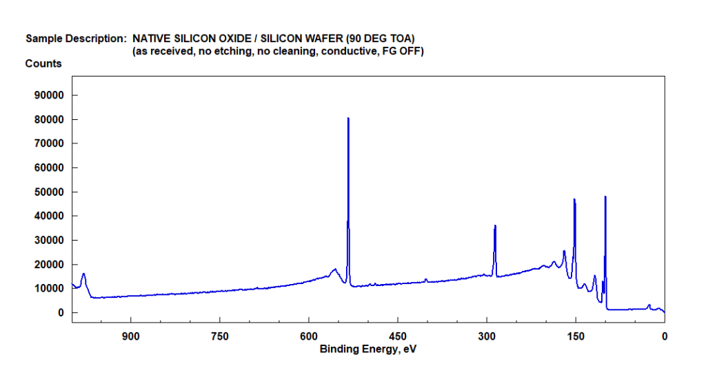
Step 1. Use the software to Manually Find and Integrate all of the Significant Peaks.
Note: Their is one very weak peak that the software did not find. Software makes a 2nd derivative to help it locate peaks. Weak peaks produce very small derivatives.
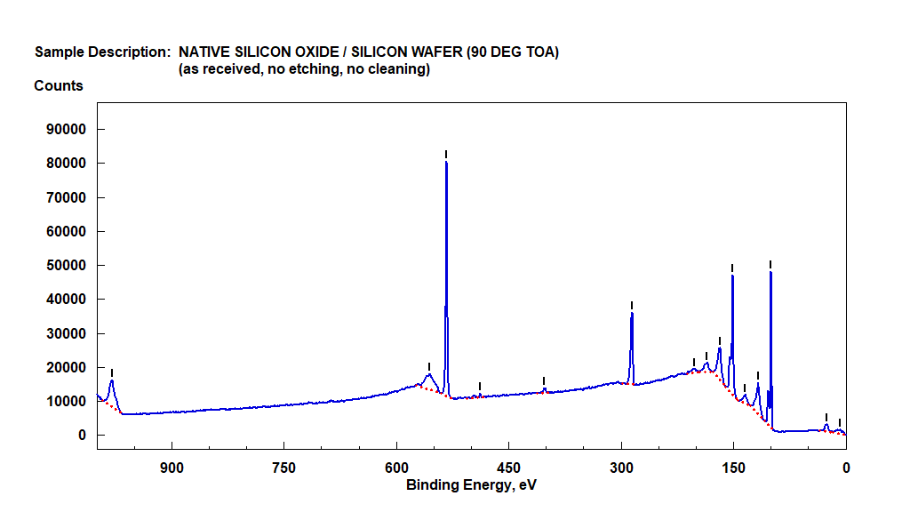
Step 2. Use the mouse to check the BEs of the peak at ~290 eV. This is C (1s).

Step 3. Use Manual Peak Identification to add the label for Carbon. “C (1s)”
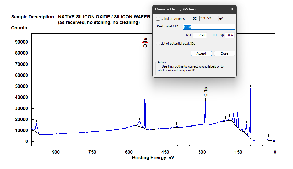
Step 4. Use the mouse pointer to locate a peak near ~530 eV. This is O (1s).

Step 5. Use the Manual Peak Identification to add the label for Oxygen. “O (1s)”
Step 6. Use the “XPS Spectral Lines” routine to identify the other significant peaks. This routine provides full XPS Peak IDs to help you label all peaks for ech element.
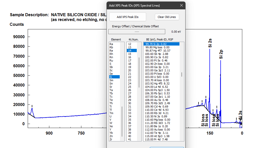
Step 7. Use Manual Identify to identify and label peaks that you remember. N (1s)
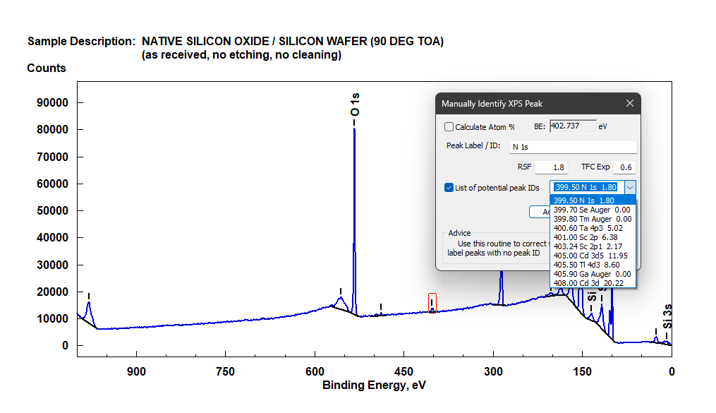
Step 8. Vertically expand the spectrum to locate very weak peaks. Such as: F (1s)
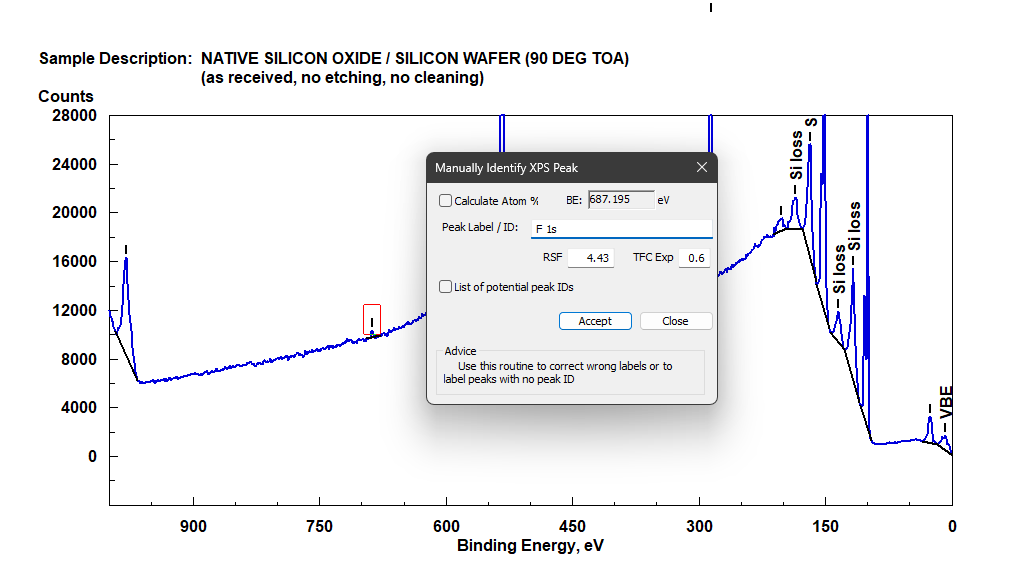
Step 9. Vertically expand. Locate and Identify other weak signals such as Sn (3d)
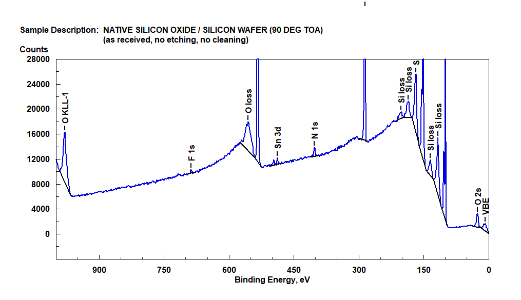
Step 10. Review the labelling. Does it match what you expected? Is it reasonable?
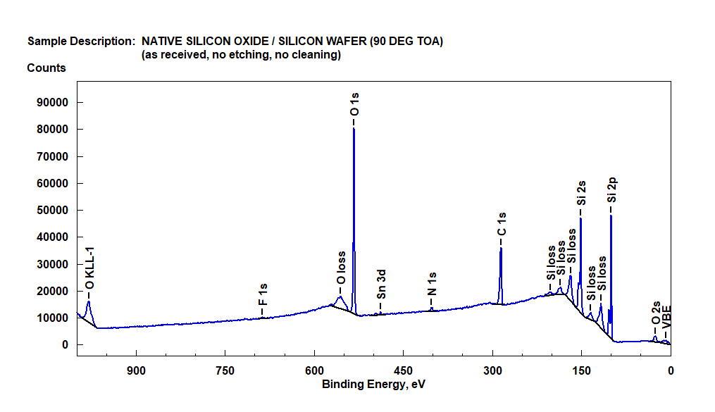
Step 11. Open the Atom% Table routine. Add a Check to the boxes of the Principle Peaks to generate Atom% table on the plot. (There is an option to hide the plot.)

Final Product. Fully labelled Survey Spectrum with Atom% Table. Save all to disk.
In this case, Nitrogen, Fluorine, and Tin were not expected. Because the peaks are small, we consider them to be low level or trace level contaminants.

In Summary: Because Carbon and Oxygen are present on every sample, we locate and label the peaks that belong to Carbon and Oxygen. The labels are: C (1s) and O (1s). After finding and labelling those always present contaminants, we then identify the remaining peaks.